Innovation Economics #2
University of Bozen-Bolzano
May 2025
March 10, 1994 - Maui, Hawaii
Mark Whitacre (Archer Daniels Midland Co.):
«I think [raising the price to] 3.55 is a little heavy right now…»Kanji Mimoto (Ajinomoto Co.):
«From now.»Mark Whitacre (Archer Daniels Midland Co.):
«In my opinion.»Kanji Mimoto (Ajinomoto Co.):
«From now.»Mark Whitacre (Archer Daniels Midland Co.):
«Right. From tomorrow, from tomorrow.»
Enter collusion
The efficacy of a market is generally thought to be rooted in competition.
- In striving to attract customers, firms are led to charge lower prices and deliver better products and services.
Collusion, whereby firms agree not to compete with one another and charge high prices, undermines this process most fundamentally.
Collusion is generally condemned by economists and policy-makers and is unlawful in almost all countries.
The lysine price-fixing conspiracy
On July 19, 1999, a US District Court in Illinois sentenced three managers from Archer Daniels Midland, a multinational company in the food industry, to over two years in prison for violating the Sherman Antitrust Act.
The three managers had been involved in a corporate agreement to voluntarily inflate the price of lysine, one of the most widely used additives in animal feed.
Shortly before, Archer Daniels Midland had agreed to settle by paying a $100 million fine, which at the time was the largest ever imposed for an antitrust violation.
The lysine price-fixing conspiracy (cont’d)
In total, the case involved nine companies from seven different countries, with settlements amounting to over $225 million.
The evidence presented in the Archer Daniels Midland case mostly consisted of audio and video recordings made by the FBI in 1994 at a hotel in Maui, Hawaii.
Under the pretext of a meeting of the European Feed Additives Association, representatives of the companies involved in the price-fixing scheme had agreed to significantly increase the profit margin on the production cost of lysine.
The lysine price-fixing conspiracy (cont’d)
Proving that a price increase is not due to external factors, such as higher production costs, is difficult.
Conversey, written note or an audio/video recording capturing the existence of a cartel is almost impossible to dispute.
This is why antitrust authorities have long used documentary evidence to show that rising prices in a particular sector are the result of collusive agreements.
Until AIs started setting prices, that is.
What is algorithmic collusion?
Pricing algorithms can ‘learn’ not to compete and to coordinate on high prices, even without explicit agreements and without being instructed to do so.
This harms consumers just like traditional, explicit price-fixing based on agreements among managers.
The increasing delegation of price-setting to algorithms has the potential for opening a back door through which firms might collude lawfully.
Algorithms learn to adopt collusive pricing rules without human intervention, oversight, or even knowledge.
Today’s roadmap
Review of some core concepts in microeconomics.
Introduction to the economic theory of collusion.
Some evidence on algorithmic collusion.
Consequences of algorithmic collusion for antitrust law.

Review of concepts
Demand
Demand function
Describes the relationship between how much consumers are willing to pay for a good and the quantity of the good consumed.
We will generally work with linear demand functions: \[ p = \alpha - \beta Q \qquad \alpha, \beta > 0 \]
where \(p\) and \(Q\) denote price and quantity, respectively.
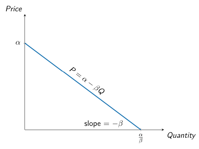
If the price is above \(\alpha\), no consumer wants to buy the good. As the price falls below \(\alpha\), demand for the good increases.
The slope of the curve is \(-\beta\): any unit increase in quantity demanded corresponds to a decrease in price equal to \(\beta\).
Each point on the demand curve represents the highest price consumers are willing to pay for a given quantity of the good.
Revenues, costs and profit
Profit
A firm’s revenue minus its total costs.
Formally, a firm’s profit is given by: \[ \pi(Q) = \underbrace{R(Q)}_{\substack{\text{Total} \\[1pt] \text{revenue}}} - \underbrace{~C(Q)}_{\substack{\text{Total} \\[1pt] \text{cost}}} \]
Revenue is: \(R(Q) = \text{market price} \times \text{quantity sold}\)
Marginal revenue and Marginal cost
Marginal revenue
The increase in total revenues when output is increased by one unit.
- Formally: \(MR(Q) = \frac{\partial R(Q)}{\partial Q}\)
Marginal cost
The increase in total cost when output is increased by one unit.
- Formally: \(MC(Q) = \frac{\partial C(Q)}{\partial Q}\)
The Bertrand model
Setup
Consider two firms, 1 and 2, that produce the same good and compete in the same market.
The two firms simultaneously choose what price to set.
They use the same technology, that is they have the same cost function: \[ C (q_i) = c q_i \qquad i = 1,2 \]
Firms’ marginal cost is constant: \(MC(q_i) = \frac{\partial C(q_i)}{\partial q_i} = c\).
The Bertrand model
Setup (cont’d)
The industry demand curve is \(p = \alpha - \beta Q\), where \(Q = q_1 + q_2\).
However, since firms compete in prices, it is convenient rewrite the demand function as: \[ Q = a - b p \]
where \(a \equiv \alpha/\beta\) and \(b \equiv 1/\beta\).
Consumers buy from the firm charging the lowest price.
The Bertrand model
Prices and demand
Take Firm 2’s perspective.
To choose its price, Firm 2 must first work out the demand for its product conditional on both its own price, \(p_2\), and Firm 1’s price, \(p_1\).
- If \(p_2 > p_1\), then Firm 2 will sell nothing.
- If \(p_2 < p_1\), then Firm 2 will supply the entire market and therefore become a monopolist.
- If \(p_2 = p_1\), then Firm 1 and Firm 2 will split the market.
Firm 2’s demand is therefore: \[ q_2 \left( p_1, p_2 \right) = \begin{cases} 0 &\text{if} \quad p_2 > p_1 \\ \frac{a - bp_2}{2} &\text{if} \quad p_2 = p_1 \\ a - bp_2 &\text{if} \quad p_2 < p_1 \\ \end{cases} \]
The Bertrand model
Profits
If \(p_2 > p_1\), then Firm 2 will sell nothing. If \(p_2 < p_1\), then Firm 2 will supply the entire market. If \(p_2 = p_1\), then Firm 1 and Firm 2 will split the market.
Firm 2’s profit is therefore: \[ \pi_2\left( p_1, p_2 \right) = \begin{cases} 0 &\text{if} \quad p_2 > p_1 \\ \left( p_2 - c \right) \frac{a - bp_2}{2} &\text{if} \quad p_2 = p_1 \\ \left( p_2 - c \right) \left( a - bp_2 \right) &\text{if} \quad p_2 < p_1 \\ \end{cases} \]
To find Firm 2’s best response function, we need to find the price \(p_2\) that maximizes \(\pi_2\left( p_1, p_2 \right)\) for any given choice of \(p_1\).
The Bertrand model
Reaction functions
If Firm 2 chooses a price just slightly lower than the price charged by Firm 1, then Firm 2 becomes a monopolist.
Firm 2 will choose the highest possible \(p_2\) lower that \(p_1\).
Firm 2’s reaction function is therefore: \[ p_2^{*} \left( p_1 \right) = \begin{cases} p_1 - \epsilon &\text{if} \quad c < p_1 < \frac{a + bc}{2b} \\ p \geq c &\text{if} \quad p_1 \leq c \\ \end{cases} \]
Similarly, Firm 1’s reaction is: \[ p_1^{*} \left( p_2 \right) = \begin{cases} p_2 - \epsilon &\text{if} \quad c < p_2 < \frac{a + bc}{2b} \\ p \geq c &\text{if} \quad p_2 \leq c \\ \end{cases} \]
The Bertrand model
Towards the equilibrium
Suppose that Firm 1 chooses a price of \(p'_1 \in \left( c, \frac{a + bc}{2b} \right)\).
By undercutting \(p'_1\), Firm 2 would serve the entire market. Firm 2’s best response to \(p'_1\) is therefore \(p'_2 = p'_1 - \varepsilon\).
Firm 1’s best response to \(p'_2\) is \(p''_1 = p'_2 - \varepsilon\).
Firm 2’s best response to \(p''_1\) is \(p''_2 = p''_1 - \varepsilon\).
…and so on.
The Bertrand model
Towards the equilibrium (cont’d)
The incentive to undercut the competitor’s price disappears when no firm can lower its price any further, that is when price equals marginal cost.
Remark: The reasoning behind undercutting occurs exclusively in the minds of the firms. Prices are actually set simultaneously.
The Bertrand model
The Bertrand-Nash equilibrium
With homogeneous products and identical constant marginal costs, the only Nash Equilibrium of the Bertrand model is: \[ p_1^{BN} = p_2^{BN} = p^{BN} = c \]
The resulting profits are: \(\pi_1^{BN} = \pi_2^{BN} = \pi^{BN} = 0\).
This counter-intuitive result is known as Bertrand Paradox.
Betrand paradox
With homogeneous products and identical constant marginal costs, two firms that simultaneously set their price to maximize profits end up earning a profit of zero.
The Bertrand model
The Bertrand-Nash equilibrium (cont’d)
To check that \(p^{BN} = c\) is a Nash equilibrium, ask whether either firm would have any incentive to change its price.
If Firm 1 raised its price (i.e. \(p_1^{BN} > c = p_2^{BN}\)), then it would then lose all of its sales to Firm 2 and therefore be no better off.
If, instead, Firm 1 lowered its price (i.e. \(p_1^{BN} < c = p_2^{BN}\)), then it would capture the entire market but would lose money on every unit it produced. Again, it would be worse off.
Thus, Firm 1 (and likewise Firm 2) has no incentive to deviate: it is doing the best it can to maximize profit, given what its competitor is doing.
An introduction to the theory of collsion
One-shot collusion
If the two firms decided to collude by raising their prices at the same time, each would see an increase in profits.
The best outcome they could achieve would be the one that maximizes the firms’ combined profit, \[ \pi(p) = (p - c) Q(p) = (p - c)(a - bp) \]
By doing so, the two firms would essentially act as a single monopolist.
The one-shot collusive outcome
We use the superscript \(C\) to denote collusion.
From the first-order condition \(\partial \pi (p) / \partial p = 0\) we obtain: \[ p_i^C = p_j^C = p^C = \frac{a + bc}{2b}\]
In this case, each firm’s profit would be half of the monopoly profit: \[ \pi_i^C = \pi_j^C = \pi^C = \frac{\left(a - bc\right)^2}{8b} \]
This profit clearly exceeds the Bertrand-Nash equilibrium profit.
The one-shot collusive outcome (cont’d)
The collusive outcome isn’t stable.
Each firm has an incentive to undercut the collusive price \(p^C\) by a tiny amount, say \(p^C - \varepsilon\).
This slightly lower price would attract all consumers to the firm that deviates, allowing it to earn monopoly-level profits, while the other firm would earn nothing.
The best response to this undercutting is to drop the price even further, and so on, until the price eventually falls to marginal cost.
The folk theorem
To get around the Bertrand paradox, we drop the assumption of a one-shot interaction and instead assume that the game can be repeated potentially infinitely many times.
Specifically, we assume that after each round of the game, there’s a probability \(\delta \in \left(0, 1 \right]\) that the game continues for another round.
The idea behind the so-called folk theorem is that firms can adopt punishment strategies which, combined with the prospect of earning a steady stream of collusive profits, serve as a strong deterrent against deviating from the collusive behavior.
The folk theorem
Friedman’s contribution
- The best-known version of the folk theorem is the one proposed by Friedman (1971):
- In the first period, choose the price \(p^C\).
- In each following period \(t > 1\), choose the price \(p^C\) if and only if both firms chose \(p^C\) in the previous period (\(t-1\)). If not, choose the Bertrand-Nash price \(p^{BN}\).
The folk theorem
Friedman’s contribution (cont’d)
- The idea:
- Firms collude for as long as neither of them deviates.
- As soon as one does, both switch to playing the Bertrand-Nash strategy from the next period onward.
- The punishment one firm — say, firm 1 — imposes on Firm 2 is to drive Firm 1’s profit down to zero, while Firm 1 is doing exactly the same to firm 2.
Friedman’s theorem
Expected profit flow under collusion
Over an infinite horizon, each firm expects to earn: \[ \Pi^c = \sum_{t=1}^\infty \pi^C \delta^{t-1} = \frac{\left(a - bc\right)^2}{8b \left( 1 - \delta \right)} \]
Mathematically, this is a geometric series with discount factor of \(\delta\).
The closed-form expression follows from: \(\sum_{t=1}^\infty \delta^{t-1} = \sum_{t=0}^\infty \delta^{t} = \frac{1}{1-\delta}\).
Friedman’s theorem
Expected profit under deviation from collusion
If a firm deviates from the collusive strategy and chooses a lower price, then it will earn the monopoly profit \(\pi^M = 2 \pi^C\) for one period.
However, from the next period onward, it will earn zero profit due to the punishment strategy adopted by the rival firm.
Friedman’s theorem
Incentive to collude
Firms will have an incentive to collude if and only if the future payoff flow is sufficiently large: \[ \Pi^C \geq 2 \pi^C \Leftrightarrow \frac{\left(a - bc\right)^2}{8b \left( 1 - \delta \right)} \geq \frac{\left(a - bc\right)^2}{4b} \]
This condition holds when \(\delta \in \left[\frac{1}{2}, 1\right]\), i.e. when the probability of the interaction continuing over time is sufficiently high.
Stability of collusion
Incentive to collude (cont’d)
The folk theorem formalizes a very intuitive idea: collusion is stable when it’s profitable enough.
In Friedman’s model, this comes at the cost of infinitely long and unrealistically harsh punishments, leaving no room for renegotiating the collusive agreement.
In practice, it’s more realistic to assume that firms may eventually abandon the costly punishment phase and return to raising prices above the competitive level.
This can also be the case when it’s AIs, rather than humans, engaging in collusion.
Evidence on algorithmic collusion
Algorithms trained on historical data
The first generation of pricing algorithms followed adaptive rules pre-set by programmers.
These algorithms typically worked by analyzing past market data to estimate the demand curve.
Based on that demand estimate and how competitors had behaved in the past, they would then pick the price that would maximize profits.
This approach was common to many other algorithms trained on human data — such as AlphaGo, the AI developed by Google DeepMind to play the board game Go, which was able to defeat Go master Lee Sedol.
Algorithms trained on historical data
The new generation of algorithms
Current algorithms can learn entirely on their own, without requiring any prior data.
They are trained completely from scratch, starting from random behaviour.
Once the AI is told what goal to aim for (e.g. profit maximization) and how often it is allowed to test out new strategies (e.g. new prices), it independently learns the strategy that best helps it reach that goal.
The new generation of algorithms
Algorithmic pricing
Recent price-setting algorithms often follow the logic of reinforcement learning (Calvano, Calzolari, Denicolò, and Pastorello 2020)
In a nutshell, this means that the AI tends to choose prices which, based on its own experience, are likely to maximize expected profits.
Every so often, the AI will try out new pricing strategies to see how they perform. If a price tested during one of these trial runs (usually picked at random from a set range) leads to higher profits, the AI will keep using it in the future.
To read the paper, click HERE.
Algorithmic pricing and collusion
The ability of algorithms to learn through experimentation makes it likely that, over time, the AIs will figure out that profit is maximized by coordinating on the collusive price, \(p^C\).
The ability to stick to the collusive path depends on being able to punish those who deviates from it. The faster the reaction, the smaller the incentive to deviate.
- That is, AIs need real-time information about the prices chosen by other firms.
- This kind of information is no longer hard to access. See e.g. Amazon’s API Gateway, which lets users monitor the price of all products sold on Amazon.
Algorithmic pricing: evidence
Evidence from a virtual market
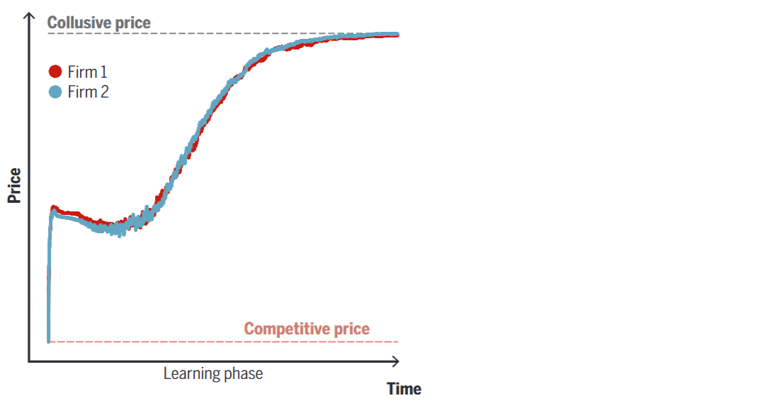
Calvano et al. (2020; 2020) programmed two identical algorithms and made them compete against each other in a virtual market.
The starting price for each algorithm, chosen arbitrarily by the authors, was the Bertrand-Nash price, \(p^{BN}\).
The AIs were instructed to maximize profits over an infinite time horizon.
Right away, they began experimenting with new strategies and reacting to each other’s choices.
Algorithmic pricing: evidence
Evidence from a virtual market (cont’d)
- As a result, prices gradually increased until they reached the collusive level, \(p^C\).
Algorithmic pricing: evidence
Evidence from a virtual market (cont’d)
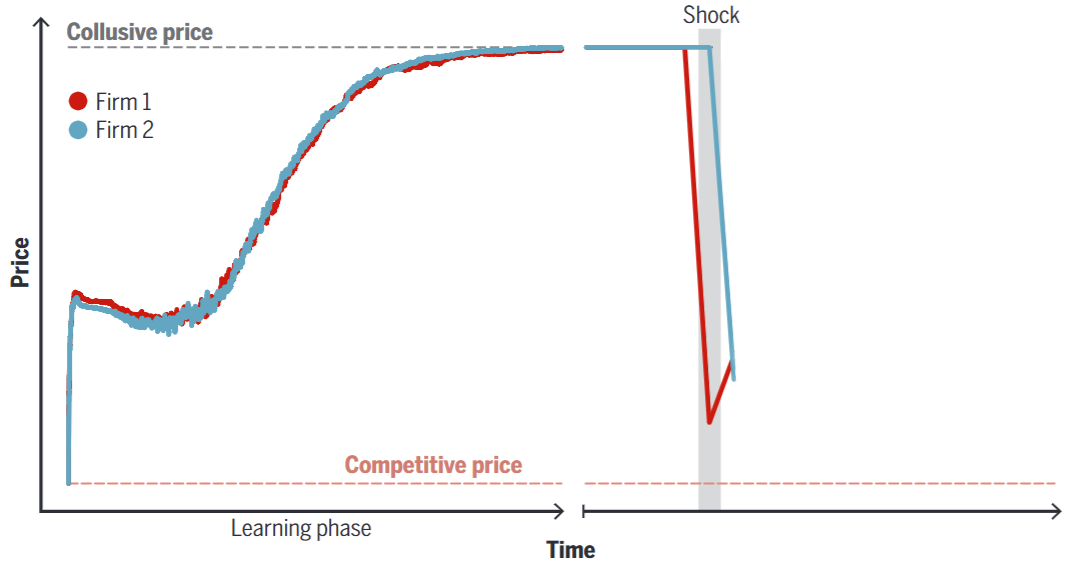
To understand whether the two AIs had truly learned to collude, Calvano and co-authors forced one of them to drastically cut its price during a specific round.
Control was then handed back to the AI starting from the following round.
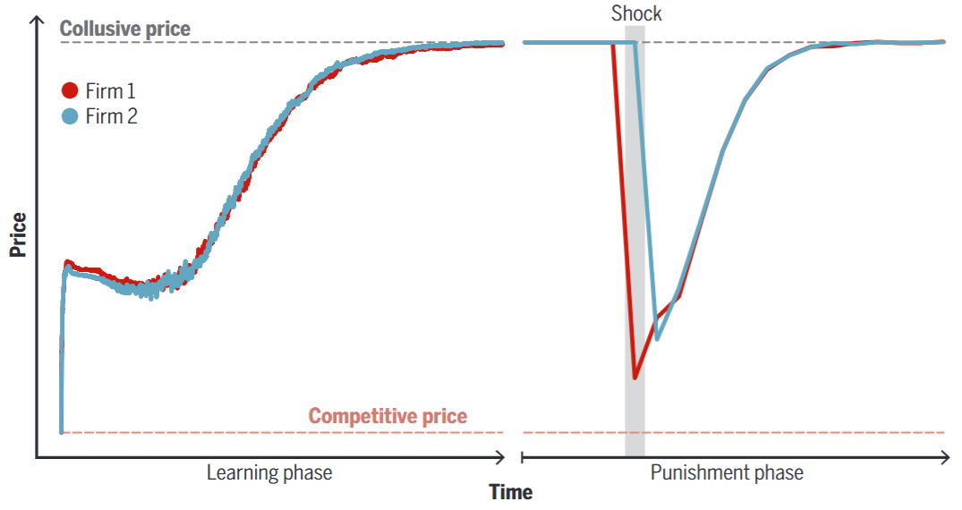
This sudden price drop triggered an immediate reaction from the rival AI, causing a sharp fall in prices — just as the folk theorem predicts as punishment.
Algorithmic pricing: evidence
Evidence from a virtual market (cont’d)
However, because the algorithms learn through experimentation, they quickly recognized how costly a prolonged price war would be.
As a result, they soon began raising prices again, eventually returning to the pre-shock level.
Algorithmic pricing: evidence
Evidence from the gasoline market
Calvano et al.’s findings were produced in a controlled environment. Do these results have external validity?
Yes they do, as shown by Assad et al. (2024) in the context of the German gasoline market.
In the summer of 2017, the Danish company a2i launched an algorithmic pricing software for gasoline in Germany.
After its introduction, gas stations using the software saw a significant increase in profit margins.
To read the paper, click HERE.
Algorithmic pricing: evidence
Evidence from the gasoline market
Stations in highly competitive areas that adopted the software experienced an average markup increase of 9%.
Stations operating in duopoly conditions (i.e. areas with only two stations) saw their markup rise by over 30%.
Meanwhile, stations with no nearby competitors showed no change in markup — since they were already charging monopoly-level prices.
This strongly suggests that the rise in profit margins was due to algorithmic collusion, not to other factors.
Algorithmic collusion and antitrust law
US antitrust regulation
The Sherman act
US antitrust law has deep roots, dating back to the Sherman Act (1890) and the Clayton Act (1914).
The Sherman Act explicitly bans anti-competitive agreements, stating in Section 1 that: “Every contract, combination in the form of trust or other- wise, or conspiracy, in restraint of trade or commerce among the several States, or with foreign nations, is hereby declared to be illegal.”
US antitrust regulation
The rule of reason and the per se rule
- Over time, US Supreme Court rulings have helped shape a body of case law that tries to balance two different principles:
Rule of reason: This approach requires courts to evaluate the actual effects of a business practice. An agreement or action is only considered illegal if it leads to reduced competition or harms market efficiency.
Per se rule: Some actions are considered automatically illegal, regardless of their actual impact on the market.
The idea is that these practices are so clearly harmful to competition that no further analysis is needed
US antitrust regulation
Price fixing and the per se rule
Currently, and for several decades now, price-fixing agreements have been judged under a strict application of the per se rule.
One of the most important cases is United States v. Socony-Vacuum Oil (1940), in which the Supreme Court ruled that: “Whatever economic justification particular price-fixing agreements may be thought to have, the law does not permit an inquiry into their reasonableness. They are all banned.”
More recently, in Arizona v. Maricopa County Medical Society (1982), the Court reaffirmed that: “The anticompetitive potential in all price-fixing agreements justifies their facial invalidation even if procompetitive justifications are offered for some.”
EU antitrust regulation
The Treaty of Rome
Similar features to US antitrust law can be found in the Treaty of Rome (1957), which later became part of the Treaty on the Functioning of the European Union (TFEU) and the Agreement on the European Economic Area (EEA).
Article 85 of the Treaty of Rome, Article 101 of the TFEU, and Article 53 of the EEA state that: “The following shall be prohibited as incompatible with the internal market: all agreements between undertakings, decisions by associations of undertakings and concerted practices which may affect trade between Member States and which have as their object or effect the prevention, restriction or distortion of competition within the internal market, and in particular those which directly or indirectly fix purchase or selling prices or any other trading conditions; […]
EU antitrust regulation
The Bonduelle - Conserve Italia case
A recent, emblematic case of price-fixing involved Conserve Italia and Bonduelle, which were found guilty by the European Commission of forming a cartel in the canned vegetable market between 2000 and 2013.
A series of unannounced inspections provided the Commission with evidence of frequent meetings between the managers of both companies, often held in private homes, where “individuals were referred to by codenames, communicated using prepaid mobile telephones or private email addresses, and exchanged information using dedicated laptops and USB keys.”
EU antitrust regulation
The Treaty of Rome (cont’d)
The third paragraph of Articles 101 TFEU and 53 EEA introduces a reasonableness clause.
Unlike the US per se rule, Paragraph 3 states that the provisions of Paragraph 1 may be declared inapplicable if they “contribute to improving the production or distribution of products or to promoting technical or economic progress.”
How to regulate algorithmic collusion?
The US case
A violation of the Sherman Act is recognized in situations where firms have “a unity of purpose or a common design and understanding, or a meeting of minds in an unlawful arrangement” (American Tobacco v. United States, 1946).
This principle, repeatedly affirmed by the Supreme Court, requires that “there must be direct or circumstantial evidence that reasonably tends to prove that the manufacturer and others had a conscious commitment to a common scheme designed to achieve an unlawful objective” (Monsanto v. Spray-Rite Services, 1984).
How to regulate algorithmic collusion?
The US case
Moreover, “There must be evidence that tends to exclude the possibility that the manufacturer and distributors were acting independently” (Monsanto v. Spray-Rite Services, 1984).
Cases where simultaneous price movements are due to independent strategic choices fall under the category of tacit collusion, which is not governed by any agreement and escape antitrust violation laws (Page 2017).
To read the paper, click Here.
How to regulate algorithmic collusion?
The US case (cont’d)
It is immediately clear that this legal approach makes it difficult to protect markets from algorithmic collusion.
Algorithms that take their own decisions without external communication and based on publicly available information, and which decide to coordinate on the collusive price \(p^C\) without specific instructions, are not violating the Sherman Act.
How to regulate algorithmic collusion?
The US case (cont’d)
According to Calvano et al. (2020), a potentially relevant common law precedent is United States v. Coscia (2017), in which the defendant was convicted for using financial trading algorithms to inflate or deflate the commodity market for speculative purposes.
Hoever, there are two issues that Calvano and co-authors seem to overlook:
- Coscia was convicted for violating the Dodd-Frank Act, not the Sherman Act. Thus, it’s not guaranteed that this ruling can serve as a precedent for collusion cases.
- In the trial, a software developer testified that Coscia specifically asked him to make the algorighm “act like a decoy which would be used to pump the market.”
As a result, the ruling may not be applicable in cases where the algorithm is not programmed with the explicit goal of committing an illegal act (like in the Coscia case), but is instead left free to learn the most profitable course of action.
How to regulate algorithmic collusion?
The EU case
European regulations face similar issues, as algorithmic collusion could potentially bypass the protection offered by Article 101 TFEU.
For example, in a reform proposal made by the European Commission in 2020, it is acknowledged that there are structural competition problems that these rules cannot tackle, such as “the increased risk for tacit collusion […] due to algorithm-based technological solutions (which are becoming increasingly prevalent across sectors).”
How to regulate algorithmic collusion?
No clear solution yet ☹️
- Calvano et al. (2020): ban entire families of altorithms altogether.
- In the US this could be possible under Section 5 of the Federal Trade Commission Act, which prohibits unfair and deceptive business practices.
- However, this approach might run into problems with the constant development of new algorithms that could be quite different from the ones that are banned, allowing them to slip through the cracks and making it necessary to update the law regularly
How to regulate algorithmic collusion?
No clear solution yet ☹️ (cont’d)
- Calvano et al. (2020): in markets where pricing algorithms are common, antitrust authorities authorities could investigate whenever price trends seem suspicious.
- For example, in the case of synchronized price increases followed by sudden decreases, which could be signs of punitive behaviour for straying from a collusive path.
- Firms’ pricing algorithms can be audited and tested to understand whether they are adopting retaliatory pricing rules.
How to regulate algorithmic collusion?
No clear solution yet ☹️ (cont’d)
- Harrington Jr. (2019): Make firms legally responsible for the pricing rules that their algorithms adopt.
- The idea: When a firm chooses to use an AI to maximize profits, and has it monitor and react to the behavior of its competitors — perhaps even knowing (or making an educated guess) that they are doing the same — it is voluntarily contributing to the potential for algorithmic collusion in the market.
- Holding firms accountable for their algorithms may incentivize them to prevent collusion by routinely monitoring the output of their learning algorithms.